目次
正規分布(確率密度関数)
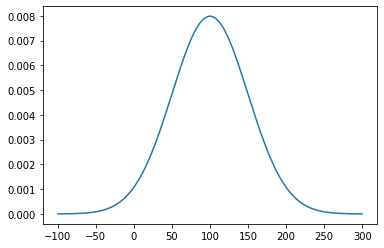
正規分布は、簡単に言うと下記の図のように中心から左右対称に山の形を描くようなグラフのこと。連続確率分布の一種で、横軸を確立変数、縦軸を確立密度と言う。下記の図で言えば、100が平均で確率密度が最も高く、平均から左右に離れていくと低くなるということ。また、正規分布のような左右対称の確率密度分布では、ある値以上になる確率を表すこともでき、例えばテストの成績で上位何%か、または下位何%かなどがわかる。
相加平均 : \(\displaystyle \mu = \frac{1}{n} \sum_{i=1}^{n}x_i\)
標準偏差 : \(\displaystyle \sigma = \sqrt{ \frac{1}{n} \sum_{i=1}^{n} (x_i – \mu)^2} \)
正規分布 : \(\displaystyle f(x) = \frac{1}{\sqrt{2 \pi \sigma^2}} \exp \left( – \frac{(x – \mu)^2}{2 \sigma^2} \right) \)
Pythonで確率密度関数を求める
NBA選手の身長で正規分布を求めてみる。データセットはKaggleでMuhammet Ali Büyüknacarさんの”2021-22 NBA Season Active NBA Players“を利用させていただく。
import math
import numpy as np
import pandas as pd
import matplotlib.pyplot as plt

def normal_distribution(x, m, s):
    # 正規分布
    exp = np.exp(-1 * ((x - m) ** 2 / (2 * s ** 2)))
    result = (1 / (np.sqrt(2 * math.pi * s ** 2))) * exp
    return result

# NBA選手
players = pd.read_csv('データセットのcsvのパス')
# フィートからセンチへ
heights = players['Height_i'] / 0.032808
# 平均値
m = heights.mean()
# 標準偏差
s = heights.std()

# 要約統計量取得
print(heights.describe())

# 160〜230cmを対象に正規分布を行う
x = range(160, 230)
y = [normal_distribution(i, m, s) for i in x]

# ヒストグラム
ax = heights.plot(kind='hist', bins=25)
ax2 = ax.twinx()
ax2.plot(x, y, color='r', linewidth=5.0)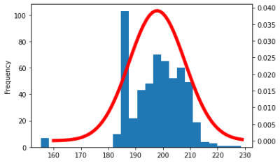
一応正規分布のような山になった。185cmあたりが突出しているが、それを除けば198cm辺りが頻出している。
scipyでの確率密度関数
scipyではnorm関数で正規分布(確率密度関数)を実装できる。
import pandas as pd
import matplotlib.pyplot as plt
from scipy.stats import norm

# NBA選手
players = pd.read_csv('データセットのcsvのパス')
# フィートからセンチへ
heights = players['Height_i'] / 0.032808
# 平均値
m = heights.mean()
# 標準偏差
s = heights.std()

# locに平均、scaleに標準偏差を指定して実行します
r = range(160, 230)
pdf = norm.pdf(r, loc=m, scale=s)

# グラフに書くとこうなります
ax = heights.plot(kind='hist', bins=25)
ax2 = ax.twinx()
ax2.plot(r, pdf, color='r', linewidth=5.0)
先程と同じ形をしている。
正規分布(累積分布関数)
確率密度関数は、ある特定の身長の確率密度、例えば身長で言えば190cmの確率密度を計算するものだったが、累積分布関数は累積の確率を計算する。つまり、身長だと170cmから220cmまでの累積の確率を計算するということ。これにより、確率変数がある値以下になる確率がわかる。また、確率密度関数では縦軸が確率密度だったが累積分布関数では縦軸が確率を表す。よって、全ての確率を足し合わせると1(100%)になる。
\(\displaystyle \mu \)は相加平均、\(\displaystyle \sigma \)は標準偏差、\(\displaystyle erf \)は誤差関数を表す。
累積分布関数 : \(\displaystyle f(x) = \frac{1}{2} \left[ 1 + erf \left( \frac{x – \mu}{\sigma \sqrt{2}} \right) \right] \)
Pythonで累積分布関数を求める
import pandas as pd
from scipy.special import erf

def normal_distribution(x, mu, sigma):
    # 累積分布関数
    result = 1 / 2 * (1 + erf((x - mu) / (sigma * math.sqrt(2))))
    return result

# NBA選手
players = pd.read_csv('/content/drive/MyDrive/nba_players.csv')
# フィートからセンチへ
heights = players['Height_i'] / 0.032808
weights = players['Weight'] / 2.2046

# 身長の平均値
height_mean = heights.mean()
# 身長の標準偏差
height_std = heights.std()
# 体重の平均値
weight_mean = weights.mean()
# 体重の標準偏差
weight_std = weights.std()

# 身長190cm以下である確率と体重90kg以下である確率
pd.DataFrame([[normal_distribution(190, height_mean, height_std)],
              [normal_distribution(90, weight_mean, weight_std)]],
             index=['身長', '体重'], columns=['確率'])

# 身長200cm以下である確率と体重100kg以下である確率
pd.DataFrame([[normal_distribution(200, height_mean, height_std)],
              [normal_distribution(100, weight_mean, weight_std)]],
             index=['身長', '体重'], columns=['確率'])
身長190cm以下である確率と体重90kg以下である確率
| 確率 | |
|---|---|
| 身長 | 0.220056 |
| 体重 | 0.235062 |
身長200cm以下である確率と体重100kg以下である確率
| 確率 | |
|---|---|
| 身長 | 0.582114 |
| 体重 | 0.569404 |
身長190cm以下である確率と体重90kg以下である確率はそれぞれ約20%程度しかないことになり、高身長で筋肉質で体重のある選手が多いこと予想できる。身長200cm以下である確率と体重100kg以下である確率はそれぞれ約58%と約56%で、これくらいになると約半数以上の選手が含まれてくることがわかる。
確率密度関数を積分する
下記の図を見ると累積分布関数は、確率密度関数を積分したもの、つまり面積と見ることもできる。これを式にすると下記のようになる。
\(\displaystyle \int_0^x \frac{1}{\sqrt{2 \pi \sigma^2}} \exp \left( – \frac{(x – \mu)^2}{2 \sigma^2} \right)dt \)
この式を用いて、先程と同じく累積分布関数を求めてみる。
import pandas as pd
from scipy.integrate import quad
from scipy.stats import norm

# NBA選手
players = pd.read_csv('/content/drive/MyDrive/nba_players.csv')
# フィートからセンチへ
heights = players['Height_i'] / 0.032808
weights = players['Weight'] / 2.2046

# 身長の平均値
height_mean = heights.mean()
# 身長の標準偏差
height_std = heights.std()
# 体重の平均値
weight_mean = weights.mean()
# 体重の標準偏差
weight_std = weights.std()

# quad(1次積分)、norm.pdf(確率密度関数)
pd.DataFrame([[quad(norm(loc=height_mean, scale=height_std).pdf, 0, 200)[0]],
              [quad(norm(loc=weight_mean, scale=weight_std).pdf, 0, 100)[0]]],
             index=['身長', '体重'], columns=['確率'])
身長200cm以下である確率と体重100kg以下である確率
| 確率 | |
|---|---|
| 身長 | 0.582114 |
| 体重 | 0.569404 |
先程と同じ結果が出力された。

記事を読んでいただきありがとうございました。